2022年4月 – 冷月梦境

2022年4月26日

window 安装composer (package not found)

打开 php 的 openssl 扩展。
浏览器访问：getcomposer.org/installer, 进入安装程序。
安装完后，composer -v 查看版本。
换镜像: composer config -g repo.packagist composer https://mirrors.aliyun.com/composer/

2022年4月13日

MathPHP

Powerful Modern Math Library for PHP

MathPHP is the only library you need to integrate mathematical functions into your applications. It is a self-contained library in pure PHP with no external dependencies.

It is actively under development with development (0.y.z) releases.

Features

Algebra
Arithmetic
Finance
Functions
- Map
- Special Functions
Information Theory
- Entropy
Linear Algebra
- Matrix
- Vector
Numbers
- Complex
- Rational
Number Theory
- Integers
Numerical Analysis
Probability
- Combinatorics
- Distributions
Sequences
- Basic
- Advanced
Set Theory
Statistics
Trigonometry

Setup

Add the library to your composer.json file in your project:

{
  "require": {
      "markrogoyski/math-php": "0.*"
  }
}

Use composer to install the library:

$ php composer.phar install

Composer will install MathPHP inside your vendor folder. Then you can add the following to your .php files to use the library with Autoloading.

require_once(__DIR__ . '/vendor/autoload.php');

Alternatively, use composer on the command line to require and install MathPHP:

$ php composer.phar require markrogoyski/math-php:0.*

Minimum Requirements

PHP 7

Usage

Algebra

use MathPHP\Algebra;

// Greatest common divisor (GCD)
$gcd = Algebra::gcd(8, 12);

// Extended greatest common divisor - gcd(a, b) = a*a' + b*b'
$gcd = Algebra::extendedGcd(12, 8); // returns array [gcd, a', b']

// Least common multiple (LCM)
$lcm = Algebra::lcm(5, 2);

// Factors of an integer
$factors = Algebra::factors(12); // returns [1, 2, 3, 4, 6, 12]

// Quadradic equation
list($a, $b, $c) = [1, 2, -8]; // x² + 2x - 8
list($x₁, $x₂)   = Algebra::quadradic($a, $b, $c);

// Cubic equation
list($a₃, $a₂, $a₁, $a₀) = [2, 9, 3, -4]; // 2x³ + 9x² + 3x -4
list($x₁, $x₂, $x₃)      = Algebra::cubic($a₃, $a₂, $a₁, $a₀);

// Quartic equation
list($a₄, $a₃, $a₂, $a₁, $a₀) = [1, -10, 35, -50, 24]; // z⁴ - 10z³ + 35z² - 50z + 24 = 0
list($z₁, $z₂, $z₃, $z₄)      = Algebra::quartic($a₄, $a₃, $a₂, $a₁, $a₀);

Arithmetic

use MathPHP\Arithmetic;

$³√x = Arithmetic::cubeRoot(-8); // -2

// Sum of digits
$digit_sum    = Arithmetic::digitSum(99):    // 18
$digital_root = Arithmetic::digitalRoot(99); // 9

// Equality of numbers within a tolerance
$x = 0.00000003458;
$y = 0.00000003455;
$ε = 0.0000000001;
$almostEqual = Arithmetic::almostEqual($x, $y, $ε); // true

// Copy sign
$magnitude = 5;
$sign      = -3;
$signed_magnitude = Arithmetic::copySign($magnitude, $sign); // -5

Finance

use MathPHP\Finance;

// Financial payment for a loan or annuity with compound interest
$rate          = 0.035 / 12; // 3.5% interest paid at the end of every month
$periods       = 30 * 12;    // 30-year mortgage
$present_value = 265000;     // Mortgage note of $265,000.00
$future_value  = 0;
$beginning     = false;      // Adjust the payment to the beginning or end of the period
$pmt           = Finance::pmt($rate, $periods, $present_value, $future_value, $beginning);

// Interest on a financial payment for a loan or annuity with compound interest.
$period = 1; // First payment period
$ipmt   = Finance::ipmt($rate, $period, $periods, $present_value, $future_value, $beginning);

// Principle on a financial payment for a loan or annuity with compound interest
$ppmt = Finance::ppmt($rate, $period, $periods, $present_value, $future_value = 0, $beginning);

// Number of payment periods of an annuity.
$periods = Finance::periods($rate, $payment, $present_value, $future_value, $beginning);

// Annual Equivalent Rate (AER) of an annual percentage rate (APR)
$nominal = 0.035; // APR 3.5% interest
$periods = 12;    // Compounded monthly
$aer     = Finance::aer($nominal, $periods);

// Annual nominal rate of an annual effective rate (AER)
$nomial = Finance::nominal($aer, $periods);

// Future value for a loan or annuity with compound interest
$payment = 1189.97;
$fv      = Finance::fv($rate, $periods, $payment, $present_value, $beginning)

// Present value for a loan or annuity with compound interest
$pv = Finance::pv($rate, $periods, $payment, $future_value, $beginning)

// Net present value of cash flows
$values = [-1000, 100, 200, 300, 400];
$npv    = Finance::npv($rate, $values);

// Interest rate per period of an annuity
$beginning = false; // Adjust the payment to the beginning or end of the period
$rate      = rate($periods, $payment, $present_value, $future_value, $beginning);

// Internal rate of return
$values = [-100, 50, 40, 30];
$irr    = Finance:irr($values); // Rate of return of an initial investment of $100 with returns of $50, $40, and $30

// Modified internal rate of return
$finance_rate      = 0.05; // 5% financing
$reinvestment_rate = 0.10; // reinvested at 10%
$mirr              = Finance:mirr($values, $finance_rate); // rate of return of an initial investment of $100 at 5% financing with returns of $50, $40, and $30 reinvested at 10%

// Discounted payback of an investment
$values  = [-1000, 100, 200, 300, 400, 500];
$rate    = 0.1;
$payback = Finance::payback($values, $rate); // The payback period of an investment with a $1,000 investment and future returns of $100, $200, $300, $400, $500 and a discount rate of 0.10

// Profitability index
$values              = [-100, 50, 50, 50];
$profitability_index = profitabilityIndex($values, $rate); // The profitability index of an initial $100 investment with future returns of $50, $50, $50 with a 10% discount rate

Functions – Map – Single Array

use MathPHP\Functions\Map;

$x = [1, 2, 3, 4];

$sums        = Map\Single::add($x, 2);      // [3, 4, 5, 6]
$differences = Map\Single::subtract($x, 1); // [0, 1, 2, 3]
$products    = Map\Single::multiply($x, 5); // [5, 10, 15, 20]
$quotients   = Map\Single::divide($x, 2);   // [0.5, 1, 1.5, 2]
$x²          = Map\Single::square($x);      // [1, 4, 9, 16]
$x³          = Map\Single::cube($x);        // [1, 8, 27, 64]
$x⁴          = Map\Single::pow($x, 4);      // [1, 16, 81, 256]
$√x          = Map\Single::sqrt($x);        // [1, 1.414, 1.732, 2]
$∣x∣         = Map\Single::abs($x);         // [1, 2, 3, 4]
$maxes       = Map\Single::max($x, 3);      // [3, 3, 3, 4]
$mins        = Map\Single::min($x, 3);      // [1, 2, 3, 3]

Functions – Map – Multiple Arrays

use MathPHP\Functions\Map;

$x = [10, 10, 10, 10];
$y = [1,   2,  5, 10];

// Map function against elements of two or more arrays, item by item (by item ...)
$sums        = Map\Multi::add($x, $y);      // [11, 12, 15, 20]
$differences = Map\Multi::subtract($x, $y); // [9, 8, 5, 0]
$products    = Map\Multi::multiply($x, $y); // [10, 20, 50, 100]
$quotients   = Map\Multi::divide($x, $y);   // [10, 5, 2, 1]
$maxes       = Map\Multi::max($x, $y);      // [10, 10, 10, 10]
$mins        = Map\Multi::mins($x, $y);     // [1, 2, 5, 10]

// All functions work on multiple arrays; not limited to just two
$x    = [10, 10, 10, 10];
$y    = [1,   2,  5, 10];
$z    = [4,   5,  6,  7];
$sums = Map\Multi::add($x, $y, $z); // [15, 17, 21, 27]

Functions – Special Functions

use MathPHP\Functions\Special;

// Gamma function Γ(z)
$z = 4;
$Γ = Special::gamma($z);          // Uses gamma definition for integers and half integers; uses Lanczos approximation for real numbers
$Γ = Special::gammaLanczos($z);   // Lanczos approximation
$Γ = Special::gammaStirling($z);  // Stirling approximation

// Incomplete gamma functions - γ(s,t), Γ(s,x)
list($x, $s) = [1, 2];
$γ = Special::lowerIncompleteGamma($x, $s); // same as γ
$γ = Special::γ($x, $s);                    // same as lowerIncompleteGamma
$Γ = Special::upperIncompleteGamma($x, $s);

// Beta function
list($x, $y) = [1, 2];
$β = Special::beta($x, $y); // same as β
$β = Special::β($x, $y);    // same as beta

// Incomplete beta functions
list($x, $a, $b) = [0.4, 2, 3];
$B  = Special::incompleteBeta($x, $a, $b);
$Iₓ = Special::regularizedIncompleteBeta($x, $a, $b);

// Multivariate beta function
$αs = [1, 2, 3];
$β  = Special::multivariateBeta($αs);

// Error function (Gauss error function)
$error = Special::errorFunction(2);              // same as erf
$error = Special::erf(2);                        // same as errorFunction
$error = Special::complementaryErrorFunction(2); // same as erfc
$error = Special::erfc(2);                       // same as complementaryErrorFunction

// Hypergeometric functions
$pFq = Special::generalizedHypergeometric($p, $q, $a, $b, $c, $z);
$₁F₁ = Special::confluentHypergeometric($a, $b, $z);
$₂F₁ = Special::hypergeometric($a, $b, $c, $z);

// Sign function (also known as signum or sgn)
$x    = 4;
$sign = Special::signum($x); // same as sgn
$sign = Special::sgn($x);    // same as signum

// Logistic function (logistic sigmoid function)
$x₀ = 2; // x-value of the sigmoid's midpoint
$L  = 3; // the curve's maximum value
$k  = 4; // the steepness of the curve
$x  = 5;
$logistic = Special::logistic($x₀, $L, $k, $x);

// Sigmoid function
$t = 2;
$sigmoid = Special::sigmoid($t);

// Softmax function
$?    = [1, 2, 3, 4, 1, 2, 3];
$σ⟮?⟯ⱼ = Special::softmax($?);

Information Theory – Entropy

use MathPHP\InformationTheory\Entropy;

// Probability distributions
$p = [0.2, 0.5, 0.3];
$q = [0.1, 0.4, 0.5];

// Shannon entropy
$bits  = Entropy::shannonEntropy($p);         // log₂
$nats  = Entropy::shannonNatEntropy($p);      // ln
$harts = Entropy::shannonHartleyEntropy($p);  // log₁₀

// Cross entropy
$H⟮p、q⟯ = Entropy::crossEntropy($p, $q);       // log₂

// Joint entropy
$P⟮x、y⟯ = [1/2, 1/4, 1/4, 0];
H⟮x、y⟯ = Entropy::jointEntropy($P⟮x、y⟯);        // log₂

// Rényi entropy
$α    = 0.5;
$Hₐ⟮X⟯ = Entropy::renyiEntropy($p, $α);         // log₂

// Perplexity
$perplexity = Entropy::perplexity($p);         // log₂

Linear Algebra – Matrix

use MathPHP\LinearAlgebra\Matrix;
use MathPHP\LinearAlgebra\MatrixFactory;

$matrix = [
    [1, 2, 3],
    [4, 5, 6],
    [7, 8, 9],
];

// Matrix factory creates most appropriate matrix
$A = MatrixFactory::create($matrix);
$B = MatrixFactory::create($matrix);

// Matrix factory can create a matrix from an array of column vectors
use MathPHP\LinearAlgebra\Vector;
$X₁ = new Vector([1, 4, 7]);
$X₂ = new Vector([2, 5, 8]);
$X₃ = new Vector([3, 6, 9]);
$C  = MatrixFactory::create([$X₁, $X₂, $X₃]);

// Can also directly instantiate desired matrix class
$A = new Matrix($matrix);
$B = new SquareMatrix($matrix);

// Basic matrix data
$array = $A->getMatrix();
$rows  = $A->getM();      // number of rows
$cols  = $A->getN();      // number of columns

// Basic matrix elements (zero-based indexing)
$row = $A->getRow(2);
$col = $A->getColumn(2);
$Aᵢⱼ = $A->get(2, 2);
$Aᵢⱼ = $A[2][2];

// Other representations of matrix data
$vectors = $A->asVectors();                // array of column vectors
$D       = $A->getDiagonalElements();      // array of the diagonal elements
$d       = $A->getSuperdiagonalElements(); // array of the superdiagonal elements
$d       = $A->getSubdiagonalElements();   // array of the subdiagonal elements

// Row operations
list($mᵢ, $mⱼ, $k) = [1, 2, 5];
$R = $A->rowInterchange($mᵢ, $mⱼ);
$R = $A->rowMultiply($mᵢ, $k);     // Multiply row mᵢ by k
$R = $A->rowAdd($mᵢ, $mⱼ, $k);     // Add k * row mᵢ to row mⱼ
$R = $A->rowExclude($mᵢ);          // Exclude row $mᵢ

// Column operations
list($nᵢ, $nⱼ, $k) = [1, 2, 5];
$R = $A->columnInterchange($nᵢ, $nⱼ);
$R = $A->columnMultiply($nᵢ, $k);     // Multiply column nᵢ by k
$R = $A->columnAdd($nᵢ, $nⱼ, $k);     // Add k * column nᵢ to column nⱼ
$R = $A->columnExclude($nᵢ);          // Exclude column $nᵢ

// Matrix operations - return a new Matrix
$A＋B  = $A->add($B);
$A⊕B   = $A->directSum($B);
$A⊕B   = $A->kroneckerSum($B);
$A−B   = $A->subtract($B);
$AB    = $A->multiply($B);
$２A   = $A->scalarMultiply(2);
$A／2  = $A->scalarDivide(2);
$−A    = $A->negate();
$A∘B   = $A->hadamardProduct($B);
$A⊗B   = $A->kroneckerProduct($B);
$Aᵀ 　 = $A->transpose();
$D  　 = $A->diagonal();
$⟮A∣B⟯  = $A->augment($B);
$⟮A∣I⟯  = $A->augmentIdentity();         // Augment with the identity matrix
$⟮A∣B⟯  = $A->augmentBelow($B);
$A⁻¹   = $A->inverse();
$Mᵢⱼ   = $A->minorMatrix($mᵢ, $nⱼ);     // Square matrix with row mᵢ and column nⱼ removed
$Mk    = $A->leadingPrincipalMinor($k); // kᵗʰ-order leading principal minor
$CM    = $A->cofactorMatrix();
$B     = $A->meanDeviation();
$S     = $A->covarianceMatrix();
$adj⟮A⟯ = $A->adjugate();

// Matrix operations - return a new Vector
$AB = $A->vectorMultiply($X₁);
$M  = $A->sampleMean();

// Matrix operations - return a value
$tr⟮A⟯   = $A->trace();
$|A|    = $a->det();              // Determinant
$Mᵢⱼ    = $A->minor($mᵢ, $nⱼ);    // First minor
$Cᵢⱼ    = $A->cofactor($mᵢ, $nⱼ);
$rank⟮A⟯ = $A->rank();

// Matrix norms - return a value
$‖A‖₁ = $A->oneNorm();
$‖A‖F = $A->frobeniusNorm(); // Hilbert–Schmidt norm
$‖A‖∞ = $A->infinityNorm();
$max  = $A->maxNorm();

// Matrix properties - return a bool
$bool = $A->isSquare();
$bool = $A->isSymmetric();
$bool = $A->isSkewSymmetric();
$bool = $A->isSingular();
$bool = $A->isNonsingular();           // Same as isInvertible
$bool = $A->isInvertible();            // Same as isNonsingular
$bool = $A->isPositiveDefinite();
$bool = $A->isPositiveSemidefinite();
$bool = $A->isNegativeDefinite();
$bool = $A->isNegativeSemidefinite();
$bool = $A->isLowerTriangular();
$bool = $A->isUpperTriangular();
$bool = $A->isTriangular();
$bool = $A->isDiagonal();
$bool = $A->isUpperBidiagonal();
$bool = $A->isLowerBidiagonal();
$bool = $A->isBidiagonal();
$bool = $A->isTridiagonal();
$bool = $A->isUpperHessenberg();
$bool = $A->isLowerHessenberg();
$bool = $A->isInvolutory();
$bool = $A->isSignature();
$bool = $A->isRef();
$bool = $A->isRref();

// Matrix decompositions
$ref  = $A->ref();                   // Row echelon form
$rref = $A->rref();                  // Reduced row echelon form
$PLU  = $A->luDecomposition();       // Returns array of Matrices [L, U, P]; P is permutation matrix
$LU   = $A->croutDecomposition();    // Returns array of Matrices [L, U]
$L    = $A->choleskyDecomposition(); // Returns lower triangular matrix L of A = LLᵀ

// Solve a linear system of equations: Ax = b
$b = new Vector(1, 2, 3);
$x = $A->solve($b);

// Map a function over each element of the Matrix
$func = function($x) {
    return $x * 2;
};
$R = $A->map($func);

// Print a matrix
print($A);
/*
 [1, 2, 3]
 [2, 3, 4]
 [3, 4, 5]
 */

// Specialized matrices
list($m, $n, $k)              = [4, 4, 2];
$identity_matrix              = MatrixFactory::identity($n);             // Ones on the main diagonal
$zero_matrix                  = MatrixFactory::zero($m, $n);             // All zeros
$ones_matrix                  = MatrixFactory::one($m, $n);              // All ones
$eye_matrix                   = MatrixFactory::eye($m, $n, $k);          // Ones (or other value) on the k-th diagonal
$exchange_matrix              = MatrixFactory::exchange($n);             // Ones on the reverse diagonal
$downshift_permutation_matrix = MatrixFactory::downshiftPermutation($n); // Permutation matrix that pushes the components of a vector down one notch with wraparound
$upshift_permutation_matrix   = MatrixFactory::upshiftPermutation($n);   // Permutation matrix that pushes the components of a vector up one notch with wraparound
$hilbert_matrix               = MatrixFactory::hilbert($n);              // Square matrix with entries being the unit fractions

// Vandermonde matrix
$V = MatrixFactory::create([1, 2, 3], 4); // 4 x 3 Vandermonde matrix
$V = new VandermondeMatrix([1, 2, 3], 4); // Same as using MatrixFactory

// Diagonal matrix
$D = MatrixFactory::create([1, 2, 3]); // 3 x 3 diagonal matrix with zeros above and below the diagonal
$D = new DiagonalMatrix([1, 2, 3]);    // Same as using MatrixFactory

// PHP Predefined Interfaces
$json = json_encode($A); // JsonSerializable
$Aᵢⱼ  = $A[$mᵢ][$nⱼ];    // ArrayAccess

Linear Algebra – Vector

use MathPHP\LinearAlgebra\Vector;

// Vector
$A = new Vector([1, 2]);
$B = new Vector([2, 4]);

// Basic vector data
$array = $A->getVector();
$n     = $A->getN();           // number of elements
$M     = $A->asColumnMatrix(); // Vector as an nx1 matrix
$M     = $A->asRowMatrix();    // Vector as a 1xn matrix

// Basic vector elements (zero-based indexing)
$item = $A->get(1);

// Vector operations - return a value
$sum  = $A->sum();
$│A│  = $A->length();           // same as l2Norm
$A⋅B  = $A->dotProduct($B);     // same as innerProduct
$A⋅B  = $A->innerProduct($B);   // same as dotProduct
$A⊥⋅B = $A->perpDotProduct($B);

// Vector operations - return a Vector or Matrix
$kA    = $A->scalarMultiply($k);
$A＋B  = $A->add($B);
$A−B   = $A->subtract($B);
$A／k  = $A->scalarDivide($k);
$A⨂B  = $A->outerProduct($B);  // Same as direct product
$AB    = $A->directProduct($B); // Same as outer product
$AxB   = $A->crossProduct($B);
$A⨂B   = $A->kroneckerProduct($B);
$Â     = $A->normalize();
$A⊥    = $A->perpendicular();
$projᵇA = $A->projection($B);   // projection of A onto B
$perpᵇA = $A->perp($B);         // perpendicular of A on B

// Vector norms - return a value
$l₁norm = $A->l1Norm();
$l²norm = $A->l2Norm();
$pnorm  = $A->pNorm();
$max    = $A->maxNorm();

// Print a vector
print($A); // [1, 2]

// PHP Predefined Interfaces
$n    = count($A);       // Countable
$json = json_encode($A); // JsonSerializable
$Aᵢ   = $A[$i];          // ArrayAccess

Number – Complex Numbers

use MathPHP\Number\Complex;

list($r, $i) = [2, 4];
$complex     = new Complex($r, $i);

// Accessors
$r = $complex->r;
$i = $complex->i;

// Unary functions
$conjugate     = $complex->complexConjugate();
$│c│           = $complex->abs();     // absolute value (modulus)
$arg⟮c⟯         = $complex->arg();     // argument (phase)
$√c            = $complex->sqrt();    // positive square root
list($z₁, $z₂) = $complex->roots();
$c⁻¹           = $complex->inverse();
$−c            = $complex->negate();
$polar         = $complex->polarForm();

// Binary functions
$c＋c = $complex->add($complex);
$c−c  = $complex->subtract($complex);
$c×c  = $complex->multiply($complex);
$c／c = $complex->divide($complex);

// Other functions
$bool   = $complex->equals($complex);
$string = (string) $complex;

Number – Rational Numbers

use MathPHP\Number\Rational;

$whole       = 0;
$numerator   = 2;
$denominator = 3;

$rational = new Rational($whole, $numerator, $denominator); // ²/₃

// Unary functions
$│rational│ = $rational->abs();

// Binary functions
$sum      = $rational->add($rational);
$diff     = $rational->subtract($rational);
$product  = $rational->multiply($rational);
$quotient = $rational->divide($rational);

// Other functions
$bool   = $rational->equals($rational);
$float  = $rational->toFloat();
$string = (string) $rational;

Number Theory – Integers

use MathPHP\NumberTheory\Integer;

$n = 225;

// Prime factorization
$factors = Integer::primeFactorization($n);

// Perfect powers
$bool        = Integer::isPerfectPower($n);
list($m, $k) = Integer::perfectPower($n);

// Coprime
$bool = Integer::coprime(4, 35);

// Even and odd
$bool = Integer::isEven($n);
$bool = Integer::isOdd($n);

Numerical Analysis – Interpolation

use MathPHP\NumericalAnalysis\Interpolation;

// Interpolation is a method of constructing new data points with the range
// of a discrete set of known data points.
// Each integration method can take input in two ways:
// 1) As a set of points (inputs and outputs of a function)
// 2) As a callback function, and the number of function evaluations to
// perform on an interval between a start and end point.

// Input as a set of points
$points = [[0, 1], [1, 4], [2, 9], [3, 16]];

// Input as a callback function
$f⟮x⟯ = function ($x) {
    return $x**2 + 2 * $x + 1;
};
list($start, $end, $n) = [0, 3, 4];

// Lagrange Polynomial
// Returns a function p(x) of x
$p = Interpolation\LagrangePolynomial::interpolate($points);                // input as a set of points
$p = Interpolation\LagrangePolynomial::interpolate($f⟮x⟯, $start, $end, $n); // input as a callback function

$p(0) // 1
$p(3) // 16

// Nevilles Method
// More accurate than Lagrange Polynomial Interpolation given the same input
// Returns the evaluation of the interpolating polynomial at the $target point
$target = 2;
$result = Interpolation\NevillesMethod::interpolate($target, $points);                // input as a set of points
$result = Interpolation\NevillesMethod::interpolate($target, $f⟮x⟯, $start, $end, $n); // input as a callback function

// Newton Polynomial (Forward)
// Returns a function p(x) of x
$p = Interpolation\NewtonPolynomialForward::interpolate($points);                // input as a set of points
$p = Interpolation\NewtonPolynomialForward::interpolate($f⟮x⟯, $start, $end, $n); // input as a callback function

$p(0) // 1
$p(3) // 16

// Natural Cubic Spline
// Returns a piecewise polynomial p(x)
$p = Interpolation\NaturalCubicSpline::interpolate($points);                // input as a set of points
$p = Interpolation\NaturalCubicSpline::interpolate($f⟮x⟯, $start, $end, $n); // input as a callback function

$p(0) // 1
$p(3) // 16

// Clamped Cubic Spline
// Returns a piecewise polynomial p(x)

// Input as a set of points
$points = [[0, 1, 0], [1, 4, -1], [2, 9, 4], [3, 16, 0]];

// Input as a callback function
$f⟮x⟯ = function ($x) {
    return $x**2 + 2 * $x + 1;
};
$f’⟮x⟯ = function ($x) {
    return 2*$x + 2;
};
list($start, $end, $n) = [0, 3, 4];

$p = Interpolation\ClampedCubicSpline::interpolate($points);                // input as a set of points
$p = Interpolation\ClampedCubicSpline::interpolate($f⟮x⟯, $f’⟮x⟯, $start, $end, $n); // input as a callback function

$p(0) // 1
$p(3) // 16

Numerical Analysis – Numerical Differentiation

use MathPHP\NumericalAnalysis\NumericalDifferentiation;

// Numerical Differentiation approximates the derivative of a function.
// Each Differentiation method can take input in two ways:
// 1) As a set of points (inputs and outputs of a function)
// 2) As a callback function, and the number of function evaluations to
// perform on an interval between a start and end point.

// Input as a callback function
$f⟮x⟯ = function ($x) {
    return $x**2 + 2 * $x + 1;
};

// Three Point Formula
// Returns an approximation for the derivative of our input at our target

// Input as a set of points
$points = [[0, 1], [1, 4], [2, 9]];

$target = 0;
list($start, $end, $n) = [0, 2, 3];
$derivative = NumericalDifferentiation\ThreePointFormula::differentiate($target, $points);                // input as a set of points
$derivative = NumericalDifferentiation\ThreePointFormula::differentiate($target, $f⟮x⟯, $start, $end, $n); // input as a callback function

// Five Point Formula
// Returns an approximation for the derivative of our input at our target

// Input as a set of points
$points = [[0, 1], [1, 4], [2, 9], [3, 16], [4, 25]];

$target = 0;
list($start, $end, $n) = [0, 4, 5];
$derivative = NumericalDifferentiation\FivePointFormula::differentiate($target, $points);                // input as a set of points
$derivative = NumericalDifferentiation\FivePointFormula::differentiate($target, $f⟮x⟯, $start, $end, $n); // input as a callback function

// Second Derivative Midpoint Formula
// Returns an approximation for the second derivative of our input at our target

// Input as a set of points
$points = [[0, 1], [1, 4], [2, 9];

$target = 1;
list($start, $end, $n) = [0, 2, 3];
$derivative = NumericalDifferentiation\SecondDerivativeMidpointFormula::differentiate($target, $points);                // input as a set of points
$derivative = NumericalDifferentiation\SecondDerivativeMidpointFormula::differentiate($target, $f⟮x⟯, $start, $end, $n); // input as a callback function

Numerical Analysis – Numerical Integration

use MathPHP\NumericalAnalysis\NumericalIntegration;

// Numerical integration approximates the definite integral of a function.
// Each integration method can take input in two ways:
// 1) As a set of points (inputs and outputs of a function)
// 2) As a callback function, and the number of function evaluations to
// perform on an interval between a start and end point.

// Trapezoidal Rule (closed Newton-Cotes formula)
$points = [[0, 1], [1, 4], [2, 9], [3, 16]];
$∫f⟮x⟯dx = NumericalIntegration\TrapezoidalRule::approximate($points); // input as a set of points

$f⟮x⟯ = function ($x) {
    return $x**2 + 2 * $x + 1;
};
list($start, $end, $n) = [0, 3, 4];
$∫f⟮x⟯dx = NumericalIntegration\TrapezoidalRule::approximate($f⟮x⟯, $start, $end, $n); // input as a callback function

// Simpsons Rule (closed Newton-Cotes formula)
$points = [[0, 1], [1, 4], [2, 9], [3, 16], [4,3]];
$∫f⟮x⟯dx = NumericalIntegration\SimpsonsRule::approximate($points); // input as a set of points

$f⟮x⟯ = function ($x) {
    return $x**2 + 2 * $x + 1;
};
list($start, $end, $n) = [0, 3, 5];
$∫f⟮x⟯dx = NumericalIntegration\SimpsonsRule::approximate($f⟮x⟯, $start, $end, $n); // input as a callback function

// Simpsons 3/8 Rule (closed Newton-Cotes formula)
$points = [[0, 1], [1, 4], [2, 9], [3, 16]];
$∫f⟮x⟯dx = NumericalIntegration\SimpsonsThreeEighthsRule::approximate($points); // input as a set of points

$f⟮x⟯ = function ($x) {
    return $x**2 + 2 * $x + 1;
};
list($start, $end, $n) = [0, 3, 5];
$∫f⟮x⟯dx = NumericalIntegration\SimpsonsThreeEighthsRule::approximate($f⟮x⟯, $start, $end, $n); // input as a callback function

// Booles Rule (closed Newton-Cotes formula)
$points = [[0, 1], [1, 4], [2, 9], [3, 16], [4, 25]];
$∫f⟮x⟯dx = NumericalIntegration\BoolesRule::approximate($points); // input as a set of points

$f⟮x⟯ = function ($x) {
    return $x**3 + 2 * $x + 1;
};
list($start, $end, $n) = [0, 4, 5];
$∫f⟮x⟯dx = NumericalIntegration\BoolesRuleRule::approximate($f⟮x⟯, $start, $end, $n); // input as a callback function

// Rectangle Method (open Newton-Cotes formula)
$points = [[0, 1], [1, 4], [2, 9], [3, 16]];
$∫f⟮x⟯dx = NumericalIntegration\RectangleMethod::approximate($points); // input as a set of points

$f⟮x⟯ = function ($x) {
    return $x**2 + 2 * $x + 1;
};
list($start, $end, $n) = [0, 3, 4];
$∫f⟮x⟯dx = NumericalIntegration\RectangleMethod::approximate($f⟮x⟯, $start, $end, $n); // input as a callback function

// Midpoint Rule (open Newton-Cotes formula)
$points = [[0, 1], [1, 4], [2, 9], [3, 16]];
$∫f⟮x⟯dx = NumericalIntegration\MidpointRule::approximate($points); // input as a set of points

$f⟮x⟯ = function ($x) {
    return $x**2 + 2 * $x + 1;
};
list($start, $end, $n) = [0, 3, 4];
$∫f⟮x⟯dx = NumericalIntegration\MidpointRule::approximate($f⟮x⟯, $start, $end, $n); // input as a callback function

Numerical Analysis – Root Finding

use MathPHP\NumericalAnalysis\RootFinding;

// Root-finding methods solve for a root of a polynomial.

// f(x) = x⁴ + 8x³ -13x² -92x + 96
$f⟮x⟯ = function($x) {
    return $x**4 + 8 * $x**3 - 13 * $x**2 - 92 * $x + 96;
};

// Newton's Method
$args     = [-4.1];  // Parameters to pass to callback function (initial guess, other parameters)
$target   = 0;       // Value of f(x) we a trying to solve for
$tol      = 0.00001; // Tolerance; how close to the actual solution we would like
$position = 0;       // Which element in the $args array will be changed; also serves as initial guess. Defaults to 0.
$x        = RootFinding\NewtonsMethod::solve($f⟮x⟯, $args, $target, $tol, $position); // Solve for x where f(x) = $target

// Secant Method
$p₀  = -1;      // First initial approximation
$p₁  = 2;       // Second initial approximation
$tol = 0.00001; // Tolerance; how close to the actual solution we would like
$x   = RootFinding\SecantMethod::solve($f⟮x⟯, $p₀, $p₁, $tol); // Solve for x where f(x) = 0

// Bisection Method
$a   = 2;       // The start of the interval which contains a root
$b   = 5;       // The end of the interval which contains a root
$tol = 0.00001; // Tolerance; how close to the actual solution we would like
$x   = RootFinding\BisectionMethod::solve($f⟮x⟯, $a, $b, $tol); // Solve for x where f(x) = 0

// Fixed-Point Iteration
// f(x) = x⁴ + 8x³ -13x² -92x + 96
// Rewrite f(x) = 0 as (x⁴ + 8x³ -13x² + 96)/92 = x
// Thus, g(x) = (x⁴ + 8x³ -13x² + 96)/92
$g⟮x⟯ = function($x) {
    return ($x**4 + 8 * $x**3 - 13 * $x**2 + 96)/92;
};
$a   = 0;       // The start of the interval which contains a root
$b   = 2;       // The end of the interval which contains a root
$p   = 0;       // The initial guess for our root
$tol = 0.00001; // Tolerance; how close to the actual solution we would like
$x   = RootFinding\FixedPointIteration::solve($g⟮x⟯, $a, $b, $p, $tol); // Solve for x where f(x) = 0

Probability – Combinatorics

use MathPHP\Probability\Combinatorics;

list($n, $x, $k) = [10, 3, 4];

// Factorials
$n！  = Combinatorics::factorial($n);
$n‼︎   = Combinatorics::doubleFactorial($n);
$x⁽ⁿ⁾ = Combinatorics::risingFactorial($x, $n);
$x₍ᵢ₎ = Combinatorics::fallingFactorial($x, $n);
$！n  = Combinatorics::subfactorial($n);

// Permutations
$nPn = Combinatorics::permutations($n);     // Permutations of n things, taken n at a time (same as factorial)
$nPk = Combinatorics::permutations($n, $k); // Permutations of n things, taking only k of them

// Combinations
$nCk  = Combinatorics::combinations($n, $k);                            // n choose k without repetition
$nC′k = Combinatorics::combinations($n, $k, Combinatorics::REPETITION); // n choose k with repetition (REPETITION const = true)

// Central binomial coefficient
$cbc = Combinatorics::centralBinomialCoefficient($n);

// Catalan number
$Cn = Combinatorics::catalanNumber($n);

// Lah number
$L⟮n、k⟯ = Combinatorics::lahNumber($n, $k)

// Multinomial coefficient
$groups    = [5, 2, 3];
$divisions = Combinatorics::multinomial($groups);

Probability – Continuous Distributions

use MathPHP\Probability\Distribution\Continuous;

// Beta distribution
$α    = 1; // shape parameter
$β    = 1; // shape parameter
$x    = 2;
$beta = new Continuous\Beta($α, $β);
$pdf  = $beta->pdf($x);
$cdf  = $beta->cdf($x);
$μ    = $beta->mean();

// Cauchy distribution
$x₀     = 2; // location parameter
$γ      = 3; // scale parameter
$x      = 1;
$cauchy = new Continuous\Cauchy(x₀, γ);
$pdf    = $cauchy->pdf(x);
$cdf    = $cauchy->cdf(x);

// χ²-distribution (Chi-Squared)
$k   = 2; // degrees of freedom
$x   = 1;
$χ²  = new Continuous\ChiSquared($k);
$pdf = $χ²->pdf($x);
$cdf = $χ²->cdf($x);

// Dirac delta distribution
$x     = 1;
$dirac = new Continuous\DiracDelta();
$pdf   = $dirac->pdf($x);
$cdf   = $dirac->cdf($x);

// Exponential distribution
$λ           = 1; // rate parameter
$x           = 2;
$exponential = new Continuous\Exponential($λ);
$pdf         = $exponential->pdf($x);
$cdf         = $exponential->cdf($x);
$μ           = $exponential->mean();

// F-distribution
$d₁  = 3; // degree of freedom v1
$d₂  = 4; // degree of freedom v2
$x   = 2;
$f   = new Continuous\F($d₁, $d₂);
$pdf = $f->pdf($x);
$cdf = $f->cdf($x);
$μ   = $f->mean();

// Gamma distribution
$k     = 2; // shape parameter
$θ     = 3; // scale parameter
$x     = 4;
$gamma = new Continuous\Gamma($k, $θ);
$pdf   = $gamma->pdf($x);
$cdf   = $gamma->cdf($x);
$μ     = $gamma->mean();

// Laplace distribution
$μ       = 1;   // location parameter
$b       = 1.5; // scale parameter (diversity)
$x       = 1;
$laplace = new Continuous\Laplace($μ, $b);
$pdf     = $laplace->pdf($x);
$cdf     = $laplace->cdf($x);

// Logistic distribution
$μ        = 2;   // location parameter
$s        = 1.5; // scale parameter
$x        = 3;
$logistic = new Continuous\Logistic($μ, $s);
$pdf      = $logistic->pdf($x);
$cdf      = $logistic->cdf($x);

// Log-logistic distribution (Fisk distribution)
$α           = 1; // scale parameter
$β           = 1; // shape parameter
$x           = 2;
$logLogistic = new Continuous\LogLogistic($α, $β);
$pdf         = $logLogistic->pdf($x);
$cdf         = $logLogistic->cdf($x);
$μ           = $logLogistic->mean();

// Log-normal distribution
$μ         = 6;   // scale parameter
$σ         = 2;   // location parameter
$x         = 4.3;
$logNormal = new Continuous\LogNormal($μ, $σ);
$pdf       = $logNormal->pdf($x);
$cdf       = $logNormal->cdf($x);
$mean      = $logNormal->mean();

// Noncentral T distribution
$ν            = 50; // degrees of freedom
$μ            = 10; // noncentrality parameter
$x            = 8;
$noncenetralT = new Continuous\NoncentralT($ν, $μ);
$pdf          = $noncenetralT->pdf($x);
$cdf          = $noncenetralT->cdf($x);
$mean         = $noncenetralT->mean();

// Normal distribution
$σ      = 1;
$μ      = 0;
$x      = 2;
$normal = new Continuous\Normal($μ, $σ);
$pdf    = $normal->pdf($x);
$cdf    = $normal->cdf($x);

// Pareto distribution
$a      = 1; // shape parameter
$b      = 1; // scale parameter
$x      = 2;
$pareto = new Continuous\Pareto($a, $b);
$pdf    = $pareto->pdf($x);
$cdf    = $pareto->cdf($x);
$μ      = $pareto->mean();

// Standard normal distribution
$z              = 2;
$standardNormal = new Continuous\StandardNormal();
$pdf            = $standardNormal->pdf($z);
$cdf            = $standardNormal->cdf($z);

// Student's t-distribution
$ν        = 3;   // degrees of freedom
$p        = 0.4; // proportion of area
$x        = 2;
$studentT = new Continuous\StudentT::pdf($ν);
$pdf      = $studentT->pdf($x);
$cdf      = $studentT->cdf($x);
$t        = $studentT->inverse2Tails($p);  // t such that the area greater than t and the area beneath -t is p

// Uniform distribution
$a       = 1; // lower boundary of the distribution
$b       = 4; // upper boundary of the distribution
$x       = 2;
$uniform = new Continuous\Uniform($a, $b);
$pdf     = $uniform->pdf($x);
$cdf     = $uniform->cdf($x);
$μ       = $uniform->mean(b);

// Weibull distribution
$k       = 1; // shape parameter
$λ       = 2; // scale parameter
$x       = 2;
$weibull = new Continuous\Weibull($k, $λ);
$pdf     = $weibull->pdf($x);
$cdf     = $weibull->cdf($x);
$μ       = $weibull->mean();

// Other CDFs - All continuous distributions
// Replace '$distribution' with desired distribution.
$inv_cdf = $distribution->inverse($target);   // Inverse CDF of the distribution
$between = $distribution->between($x₁, $x₂);  // Probability of being between two points, x₁ and x₂
$outside = $distribution->outside($x₁, $x);   // Probability of being between below x₁ and above x₂
$above   = $distribution->above($x);          // Probability of being above x to ∞

// Random Number Generator
$random  = $distribution->rand();  // A random number with a given distribution

Probability – Discrete Distributions

use MathPHP\Probability\Distribution\Discrete;

// Bernoulli distribution (special case of binomial where n = 1)
$p         = 0.3;
$k         = 0;
$bernoulli = new Discrete\Bernoulli($p);
$pmf       = $bernoulli->pmf($k);
$cdf       = $bernoulli->cdf($k);

// Binomial distribution
$n        = 2;   // number of events
$p        = 0.5; // probability of success
$r        = 1;   // number of successful events
$binomial = new Discrete\Binomial($n, $p);
$pmf      = $binomial->pmf($r);
$cdf      = $binomial->cdf($r);

// Categorical distribution
$k             = 3;                                    // number of categories
$probabilities = ['a' => 0.3, 'b' => 0.2, 'c' => 0.5]; // probabilities for categorices a, b, and c
$categorical   = new Discrete\Categorical($k, $probabilities);
$pmf_a         = $categorical->pmf('a');
$mode          = $categorical->mode();

// Geometric distribution (failures before the first success)
$p         = 0.5; // success probability
$k         = 2;   // number of trials
$geometric = new Discrete\Geometric($p);
$pmf       = $geometric->pmf($k);
$cdf       = $geometric->cdf($k);

// Hypergeometric distribution
$N        = 50; // population size
$K        = 5;  // number of success states in the population
$n        = 10; // number of draws
$k        = 4;  // number of observed successes
$hypergeo = new Discrete\Hypergeometric($N, $K, $n);
$pmf      = $hypergeo->pmf($k);
$cdf      = $hypergeo->cdf($k);
$μ        = $hypergeo->mean();

// Multinomial distribution
$frequencies   = [7, 2, 3];
$probabilities = [0.40, 0.35, 0.25];
$multinomial   = new Discrete\Multinomial($probabilities);
$pmf           = $multinomial->pmf($frequencies);

// Negative binomial distribution (Pascal)
$r                = 1;   // number of successful events
$P                = 0.5; // probability of success on an individual trial
$x                = 2;   // number of trials required to produce r successes
$negativeBinomial = new Discrete\NegativeBinomial($r, $p);
$pmf              = $negativeBinomial->pmf($x);

// Pascal distribution (Negative binomial)
$r      = 1;   // number of successful events
$P      = 0.5; // probability of success on an individual trial
$x      = 2;   // number of trials required to produce r successes
$pascal = new Discrete\Pascal($r, $p);
$pmf    = $pascal->pmf($x);

// Poisson distribution
$λ       = 2; // average number of successful events per interval
$k       = 3; // events in the interval
$poisson = new Discrete\Poisson($λ);
$pmf     = $poisson->pmf($k);
$cdf     = $poisson->cdf($k);

// Shifted geometric distribution (probability to get one success)
$p                = 0.5; // success probability
$k                = 2;   // number of trials
$shiftedGeometric = new Discrete\ShiftedGeometric($p);
$pmf              = $shiftedGeometric->pmf($k);
$cdf              = $shiftedGeometric->cdf($k);

// Uniform distribution
$a       = 1; // lower boundary of the distribution
$b       = 4; // upper boundary of the distribution
$k       = 2; // percentile
$uniform = new Discrete\Uniform($a, $b);
$pmf     = $uniform->pmf();
$cdf     = $uniform->cdf($k);
$μ       = $uniform->mean();

Probability – Multivariate Distributions

use MathPHP\Probability\Distribution\Multivariate;

// Dirichlet distribution
$αs        = [1, 2, 3];
$xs        = [0.07255081, 0.27811903, 0.64933016];
$dirichlet = new Multivariate\Dirichlet($αs);
$pdf       = $dirichlet->pdf($xs);

// Normal distribution
$μ      = [1, 1.1];
$∑      = MatrixFactory::create([
    [1, 0],
    [0, 1],
]);
$X      = [0.7, 1.4];
$normal = new Multivariate\Normal($μ, $∑);
$pdf    = $normal->pdf($X);

Probability – Distribution Tables

use MathPHP\Probability\Distribution\Table;

// Provided solely for completeness' sake.
// It is statistics tradition to provide these tables.
// MathPHP has dynamic distribution CDF functions you can use instead.

// Standard Normal Table (Z Table)
$table       = Table\StandardNormal::Z_SCORES;
$probability = $table[1.5][0];                 // Value for Z of 1.50

// t Distribution Tables
$table   = Table\TDistribution::ONE_SIDED_CONFIDENCE_LEVEL;
$table   = Table\TDistribution::TWO_SIDED_CONFIDENCE_LEVEL;
$ν       = 5;  // degrees of freedom
$cl      = 99; // confidence level
$t       = $table[$ν][$cl];

// t Distribution Tables
$table = Table\TDistribution::ONE_SIDED_ALPHA;
$table = Table\TDistribution::TWO_SIDED_ALPHA;
$ν     = 5;     // degrees of freedom
$α     = 0.001; // alpha value
$t     = $table[$ν][$α];

// χ² Distribution Table
$table = Table\ChiSquared::CHI_SQUARED_SCORES;
$df    = 2;    // degrees of freedom
$p     = 0.05; // P value
$χ²    = $table[$df][$p];

Sequences – Basic

use MathPHP\Sequence\Basic;

$n = 5; // Number of elements in the sequence

// Arithmetic progression
$d           = 2;  // Difference between the elements of the sequence
$a₁          = 1;  // Starting number for the sequence
$progression = Basic::arithmeticProgression($n, $d, $a₁);
// [1, 3, 5, 7, 9] - Indexed from 1

// Geometric progression (arⁿ⁻¹)
$a           = 2; // Scalar value
$r           = 3; // Common ratio
$progression = Basic::geometricProgression($n, $a, $r);
// [2(3)⁰, 2(3)¹, 2(3)², 2(3)³] = [2, 6, 18, 54] - Indexed from 1

// Square numbers (n²)
$squares = Basic::squareNumber($n);
// [0², 1², 2², 3², 4²] = [0, 1, 4, 9, 16] - Indexed from 0

// Cubic numbers (n³)
$cubes = Basic::cubicNumber($n);
// [0³, 1³, 2³, 3³, 4³] = [0, 1, 8, 27, 64] - Indexed from 0

// Powers of 2 (2ⁿ)
$po2 = Basic::powersOfTwo($n);
// [2⁰, 2¹, 2², 2³, 2⁴] = [1, 2, 4, 8, 16] - Indexed from 0

// Powers of 10 (10ⁿ)
$po10 = Basic::powersOfTen($n);
// [10⁰, 10¹, 10², 10³, 10⁴] = [1, 10, 100, 1000, 10000] - Indexed from 0

// Factorial (n!)
$fact = Basic::factorial($n);
// [0!, 1!, 2!, 3!, 4!] = [1, 1, 2, 6, 24] - Indexed from 0

// Digit sum
$digit_sum = Basic::digitSum($n);
// [0, 1, 2, 3, 4] - Indexed from 0

// Digital root
$digit_root = Basic::digitalRoot($n);
// [0, 1, 2, 3, 4] - Indexed from 0

Sequences – Advanced

use MathPHP\Sequence\Advanced;

$n = 6; // Number of elements in the sequence

// Fibonacci (Fᵢ = Fᵢ₋₁ + Fᵢ₋₂)
$fib = Advanced::fibonacci($n);
// [0, 1, 1, 2, 3, 5] - Indexed from 0

// Lucas numbers
$lucas = Advanced::lucasNumber($n);
// [2, 1, 3, 4, 7, 11] - Indexed from 0

// Pell numbers
$pell = Advanced::pellNumber($n);
// [0, 1, 2, 5, 12, 29] - Indexed from 0

// Triangular numbers (figurate number)
$triangles = Advanced::triangularNumber($n);
// [1, 3, 6, 10, 15, 21] - Indexed from 1

// Pentagonal numbers (figurate number)
$pentagons = Advanced::pentagonalNumber($n);
// [1, 5, 12, 22, 35, 51] - Indexed from 1

// Hexagonal numbers (figurate number)
$hexagons = Advanced::hexagonalNumber($n);
// [1, 6, 15, 28, 45, 66] - Indexed from 1

// Heptagonal numbers (figurate number)
$hexagons = Advanced::heptagonalNumber($n);
// [1, 4, 7, 13, 18, 27] - Indexed from 1

// Look-and-say sequence (describe the previous term!)
$look_and_say = Advanced::lookAndSay($n);
// ['1', '11', '21', '1211', '111221', '312211'] - Indexed from 1

// Lazy caterer's sequence (central polygonal numbers)
$lazy_caterer = Advanced::lazyCaterers($n);
// [1, 2, 4, 7, 11, 16] - Indexed from 0

// Magic squares series (magic constants; magic sums)
$magic_squares = Advanced::magicSquares($n);
// [0, 1, 5, 15, 34, 65] - Indexed from 0

// Perfect powers sequence
$perfect_powers = Advanced::perfectPowers($n);
// [4, 8, 9, 16, 25, 27] - Indexed from 0

// Not perfect powers sequence
$not_perfect_powers = Advanced::notPerfectPowers($n);
// [2, 3, 5, 6, 7, 10] - Indexed from 0

// Prime numbers up to n (n is not the number of elements in the sequence)
$primes = Advanced::primesUpTo(30);
// [2, 3, 5, 7, 11, 13, 17, 19, 23, 29] - Indexed from 0

Set Theory

use MathPHP\SetTheory\Set;
use MathPHP\SetTheory\ImmutableSet;

// Sets and immutable sets
$A = new Set([1, 2, 3]);          // Can add and remove members
$B = new ImmutableSet([3, 4, 5]); // Cannot modify set once created

// Basic set data
$set         = $A->asArray();
$cardinality = $A->length();
$bool        = $A->isEmpty();

// Set membership
$true = $A->isMember(2);
$true = $A->isNotMember(8);

// Add and remove members
$A->add(4);
$A->add(new Set(['a', 'b']));
$A->addMulti([5, 6, 7]);
$A->remove(7);
$A->removeMulti([5, 6]);
$A->clear();

// Set properties against other sets - return boolean
$bool = $A->isDisjoint($B);
$bool = $A->isSubset($B);         // A ⊆ B
$bool = $A->isProperSubset($B);   // A ⊆ B & A ≠ B
$bool = $A->isSuperset($B);       // A ⊇ B
$bool = $A->isProperSuperset($B); // A ⊇ B & A ≠ B

// Set operations with other sets - return a new Set
$A∪B  = $A->union($B);
$A∩B  = $A->intersect($B);
$A＼B = $A->difference($B);          // relative complement
$AΔB  = $A->symmetricDifference($B);
$A×B  = $A->cartesianProduct($B);

// Other set operations
$P⟮A⟯ = $A->powerSet();
$C   = $A->copy();

// Print a set
print($A); // Set{1, 2, 3, 4, Set{a, b}}

// PHP Interfaces
$n = count($A);                 // Countable
foreach ($A as $member) { ... } // Iterator

// Fluent interface
$A->add(5)->add(6)->remove(4)->addMulti([7, 8, 9]);

Statistics – ANOVA

Statistics – Averages

use MathPHP\Statistics\Average;

$numbers = [13, 18, 13, 14, 13, 16, 14, 21, 13];

// Mean, median, mode
$mean   = Average::mean($numbers);
$median = Average::median($numbers);
$mode   = Average::mode($numbers); // Returns an array — may be multimodal

// Weighted mean
$weights       = [12, 1, 23, 6, 12, 26, 21, 12, 1];
$weighted_mean = Average::weightedMean($numbers, $weights)

// Other means of a list of numbers
$geometric_mean      = Average::geometricMean($numbers);
$harmonic_mean       = Average::harmonicMean($numbers);
$contraharmonic_mean = Average::contraharmonicMean($numbers);
$quadratic_mean      = Average::quadraticMean($numbers);  // same as rootMeanSquare
$root_mean_square    = Average::rootMeanSquare($numbers); // same as quadraticMean
$trimean             = Average::trimean($numbers);
$interquartile_mean  = Average::interquartileMean($numbers); // same as iqm
$interquartile_mean  = Average::iqm($numbers);               // same as interquartileMean
$cubic_mean          = Average::cubicMean($numbers);

// Truncated mean (trimmed mean)
$trim_percent   = 25;
$truncated_mean = Average::truncatedMean($numbers, $trim_percent);

// Generalized mean (power mean)
$p                = 2;
$generalized_mean = Average::generalizedMean($numbers, $p); // same as powerMean
$power_mean       = Average::powerMean($numbers, $p);       // same as generalizedMean

// Lehmer mean
$p           = 3;
$lehmer_mean = Average::lehmerMean($numbers, $p);

// Moving averages
$n       = 3;
$weights = [3, 2, 1];
$SMA     = Average::simpleMovingAverage($numbers, $n);             // 3 n-point moving average
$CMA     = Average::cumulativeMovingAverage($numbers);
$WMA     = Average::weightedMovingAverage($numbers, $n, $weights);
$EPA     = Average::exponentialMovingAverage($numbers, $n);

// Means of two numbers
list($x, $y) = [24, 6];
$agm           = Average::arithmeticGeometricMean($x, $y); // same as agm
$agm           = Average::agm($x, $y);                     // same as arithmeticGeometricMean
$log_mean      = Average::logarithmicMean($x, $y);
$heronian_mean = Average::heronianMean($x, $y);
$identric_mean = Average::identricMean($x, $y);

// Averages report
$averages = Average::describe($numbers);
print_r($averages);
/* Array (
 [mean] => 15
 [median] => 14
 [mode] => Array ( [0] => 13 )
 [geometric_mean] => 14.789726414533
 [harmonic_mean] => 14.605077399381
 [contraharmonic_mean] => 15.474074074074
 [quadratic_mean] => 15.235193176035
 [trimean] => 14.5
 [iqm] => 14
 [cubic_mean] => 15.492307432707
) */

Statistics – Circular

use MathPHP\Statistics\Circular;

$angles = [1.51269877, 1.07723915, 0.81992282];

$θ = Circular::mean($angles);
$R = Circular::resultantLength($angles);
$ρ = Circular::meanResultantLength($angles);
$V = Circular::variance($angles);
$ν = Circular::standardDeviation($angles);

// Descriptive circular statistics report
$stats = Circular::describe($angles);
print_r($stats);
/* Array (
 [n] => 3
 [mean] => 1.1354043006436
 [resultant_length] => 2.8786207547493
 [mean_resultant_length] => 0.9595402515831
 [variance] => 0.040459748416901
 [sd] => 0.28740568481722
); */

Statistics – Correlation

use MathPHP\Statistics\Correlation;

$X = [1, 2, 3, 4, 5];
$Y = [2, 3, 4, 4, 6];

// Covariance
$σxy = Correlation::covariance($X, $Y);  // Has optional parameter to set population (defaults to sample covariance)

// Weighted covariance
$w    = [2, 3, 1, 1, 5];
$σxyw = Correlation::weightedCovariance($X, $Y, $w);

// r - Pearson product-moment correlation coefficient (Pearson's r)
$r = Correlation::r($X, $Y);  // Has optional parameter to set population (defaults to sample correlation coefficient)

// Weighted correlation coefficient
$rw = Correlation::weightedCorrelationCoefficient($X, $Y, $w);

// R² - Coefficient of determination
$R² = Correlation::r2($X, $Y);  // Has optional parameter to set population (defaults to sample coefficient of determination)

// τ - Kendall rank correlation coefficient (Kendall's tau)
$τ = Correlation::kendallsTau($X, $Y);

// ρ - Spearman's rank correlation coefficient (Spearman's rho)
$ρ = Correlation::spearmansRho($X, $Y);

// Descriptive correlation report
$stats = Correlation::describe($X, $Y);
print_r($stats);
/* Array (
 [cov] => 2.25
 [r] => 0.95940322360025
 [r2] => 0.92045454545455
 [tau] => 0.94868329805051
 [rho] => 0.975
) */

// Confidence ellipse - create an ellipse surrounding the data at a specified standard deviation
$sd           = 1;
$num_points   = 11; // Optional argument specifying number of points of the ellipse
$ellipse_data = Correlation::confidenceEllipse($X, $Y, $sd, $num_points);

Statistics – Descriptive

Statistics – Distance and Divergence

use MathPHP\Statistics\Distance;

// Probability distributions
$p = [0.2, 0.5, 0.3];
$q = [0.1, 0.4, 0.5];

// Distances
$DB⟮p、q⟯ = Distance::bhattacharyyaDistance($p, $q);
$H⟮p、q⟯  = Distance::hellingerDistance($p, $q)

// Divergences
$Dkl⟮P‖Q⟯ = Distance::kullbackLeiblerDivergence($p, $q);
$JSD⟮P‖Q⟯ = Distance::jensenShannonDivergence($p, $q);

Statistics – Distributions

use MathPHP\Statistics\Distribution;

$grades = ['A', 'A', 'B', 'B', 'B', 'B', 'C', 'C', 'D', 'F'];

// Frequency distributions (frequency and relative frequency)
$frequencies          = Distribution::frequency($grades);         // [ A => 2, B => 4, C => 2, D => 1, F => 1 ]
$relative_frequencies = Distribution::relativeFrequency($grades); // [ A => 0.2, B => 0.4, C => 0.2, D => 0.1, F => 0.1 ]

// Cumulative frequency distributions (cumulative and cumulative relative)
$cumulative_frequencies          = Distribution::cumulativeFrequency($grades);         // [ A => 2, B => 6, C => 8, D => 9, F => 10 ]
$cumulative_relative_frequencies = Distribution::cumulativeRelativeFrequency($grades); // [ A => 0.2, B => 0.6, C => 0.8, D => 0.9, F => 1 ]

// Stem and leaf plot
// Return value is array where keys are the stems, values are the leaves
$values             = [44, 46, 47, 49, 63, 64, 66, 68, 68, 72, 72, 75, 76, 81, 84, 88, 106];
$stem_and_leaf_plot = Distribution::stemAndLeafPlot($values);
// [4 => [4, 6, 7, 9], 5 => [], 6 => [3, 4, 6, 8, 8], 7 => [2, 2, 5, 6], 8 => [1, 4, 8], 9 => [], 10 => [6]]

// Optional second parameter will print stem and leaf plot to STDOUT
Distribution::stemAndLeafPlot($values, Distribution::PRINT);
/*
 4 | 4 6 7 9
 5 |
 6 | 3 4 6 8 8
 7 | 2 2 5 6
 8 | 1 4 8
 9 |
10 | 6
*/

Statistics – Effect Size

use MathPHP\Statistics\EffectSize;

$SSt = 24;  // Sum of squares treatment
$SSE = 300; // Sum of squares error
$SST = 600; // Sum of squares total
$dft = 1;   // Degrees of freedom treatment
$MSE = 18;  // Mean squares error

// η² - Eta-squared
$η²  = EffectSize::etaSquared($SSt, $SST);
$η²p = EffectSize::partialEtaSquared($SSt, $SSE);

// ω² - Omega-squared
$ω² = EffectSize::omegaSquared($SSt, $dft, $SST, $MSE);

// Cohen's ƒ²
$ƒ² = EffectSize::cohensF($η²);
$ƒ² = EffectSize::cohensF($ω²);
$ƒ² = EffectSize::cohensF($R²);

// Cohen's q
list($r₁, $r₂) = [0.1, 0.2];
$q = EffectSize::cohensQ($r₁, $r₂);

// Cohen's d
list($μ₁, $σ₁) = [6.7, 1.2];
list($μ₂, $σ₂) = [6, 1];
$d = EffectSize::cohensD($μ₁, $μ₂, $σ₁, $σ₂);

// Hedges' g
list($μ₁, $σ₁, $n₁) = [6.7, 1.2, 15];
list($μ₂, $σ₂, $n₂) = [6, 1, 15];
$g = EffectSize::hedgesG($μ₁, $μ₂, $σ₁, $σ₂, $n₁, $n₂);

// Glass' Δ
$Δ = EffectSize::glassDelta($μ₁, $μ₂, $σ₂);

Statistics – Experiments

use MathPHP\Statistics\Experiment;

$a = 28;   // Exposed and event present
$b = 129;  // Exposed and event absent
$c = 4;    // Non-exposed and event present
$d = 133;  // Non-exposed and event absent

// Risk ratio (relative risk) - RR
$RR = Experiment::riskRatio($a, $b, $c, $d);
// ['RR' => 6.1083, 'ci_lower_bound' => 2.1976, 'ci_upper_bound' => 16.9784, 'p' => 0.0005]

// Odds ratio (OR)
$OR = Experiment::oddsRatio($a, $b, $c, $d);
// ['OR' => 7.2171, 'ci_lower_bound' => 2.4624, 'ci_upper_bound' => 21.1522, 'p' => 0.0003]

// Likelihood ratios (positive and negative)
$LL = Experiment::likelihoodRatio($a, $b, $c, $d);
// ['LL+' => 7.4444, 'LL-' => 0.3626]

$sensitivity = 0.67;
$specificity = 0.91;
$LL          = Experiment::likelihoodRatioSS($sensitivity, $specificity);

Statistics – Kernel Density Estimation

use MathPHP\Statistics\KernelDensityEstimation

$data = [-2.76, -1.09, -0.5, -0.15, 0.22, 0.69, 1.34, 1.75];
$x    = 0.5;

// Density estimator with default bandwidth (normal distribution approximation) and kernel function (standard normal)
$kde     = new KernelDensityEstimation($data);
$density = $kde->evaluate($x)

// Custom bandwidth
$h = 0.1;
$kde->setBandwidth($h);

// Library of built-in kernel functions
$kde->setKernelFunction(KernelDensityEstimation::STANDARD_NORMAL);
$kde->setKernelFunction(KernelDensityEstimation::NORMAL);
$kde->setKernelFunction(KernelDensityEstimation::UNIFORM);
$kde->setKernelFunction(KernelDensityEstimation::TRIANGULAR);
$kde->setKernelFunction(KernelDensityEstimation::EPANECHNIKOV);
$kde->setKernelFunction(KernelDensityEstimation::TRICUBE);

// Set custom kernel function (user-provided callable)
$kernel = function ($x) {
  if (abs($x) > 1) {
      return 0;
  } else {
      return 70 / 81 * ((1 - abs($x) ** 3) ** 3);
  }
};
$kde->setKernelFunction($kernel);

// All customization optionally can be done in the constructor
$kde = new KernelDesnsityEstimation($data, $h, $kernel);

Statistics – Random Variables

use MathPHP\Statistics\RandomVariable;

$X = [1, 2, 3, 4];
$Y = [2, 3, 4, 5];

// Central moment (nth moment)
$second_central_moment = RandomVariable::centralMoment($X, 2);
$third_central_moment  = RandomVariable::centralMoment($X, 3);

// Skewness (population and sample)
$skewness = RandomVariable::skewness($X);            // general method of calculating skewness
$skewness = RandomVariable::populationSkewness($X);  // similar to Excel's SKEW.P
$skewness = RandomVariable::sampleSkewness($X);      // similar to Excel's SKEW
$SES      = RandomVariable::ses(count($X));          // standard error of skewness

// Kurtosis (excess)
$kurtosis    = RandomVariable::kurtosis($X);
$platykurtic = RandomVariable::isPlatykurtic($X); // true if kurtosis is less than zero
$leptokurtic = RandomVariable::isLeptokurtic($X); // true if kurtosis is greater than zero
$mesokurtic  = RandomVariable::isMesokurtic($X);  // true if kurtosis is zero
$SEK         = RandomVariable::sek(count($X));    // standard error of kurtosis

// Standard error of the mean (SEM)
$sem = RandomVariable::standardErrorOfTheMean($X); // same as sem
$sem = RandomVariable::sem($X);                    // same as standardErrorOfTheMean

// Confidence interval
$μ  = 90; // sample mean
$n  = 9;  // sample size
$σ  = 36; // standard deviation
$cl = 99; // confidence level
$ci = RandomVariable::confidenceInterval($μ, $n, $σ, $cl); // Array( [ci] => 30.91, [lower_bound] => 59.09, [upper_bound] => 120.91 )

Statistics – Regressions

use MathPHP\Statistics\Regression;

$points = [[1,2], [2,3], [4,5], [5,7], [6,8]];

// Simple linear regression (least squares method)
$regression = new Regression\Linear($points);
$parameters = $regression->getParameters();          // [m => 1.2209302325581, b => 0.6046511627907]
$equation   = $regression->getEquation();            // y = 1.2209302325581x + 0.6046511627907
$y          = $regression->evaluate(5);              // Evaluate for y at x = 5 using regression equation
$ci         = $regression->ci(5, 0.5);               // Confidence interval for x = 5 with p-value of 0.5
$pi         = $regression->pi(5, 0.5);               // Prediction interval for x = 5 with p-value of 0.5; Optional number of trials parameter.
$Ŷ          = $regression->yHat();
$r          = $regression->r();                      // same as correlationCoefficient
$r²         = $regression->r2();                     // same as coefficientOfDetermination
$se         = $regression->standardErrors();         // [m => se(m), b => se(b)]
$t          = $regression->tValues();                // [m => t, b => t]
$p          = $regression->tProbability();           // [m => p, b => p]
$F          = $regression->fStatistic();
$p          = $regression->fProbability();
$h          = $regression->leverages();
$e          = $regression->residuals();
$D          = $regression->cooksD();
$DFFITS     = $regression->dffits();
$SStot      = $regression->sumOfSquaresTotal();
$SSreg      = $regression->sumOfSquaresRegression();
$SSres      = $regression->sumOfSquaresResidual();
$MSR        = $regression->meanSquareRegression();
$MSE        = $regression->meanSquareResidual();
$MSTO       = $regression->meanSquareTotal();
$error      = $regression->errorSd();                // Standard error of the residuals
$V          = $regression->regressionVariance();
$n          = $regression->getSampleSize();          // 5
$points     = $regression->getPoints();              // [[1,2], [2,3], [4,5], [5,7], [6,8]]
$xs         = $regression->getXs();                  // [1, 2, 4, 5, 6]
$ys         = $regression->getYs();                  // [2, 3, 5, 7, 8]
$ν          = $regression->degreesOfFreedom();

// Linear regression through a fixed point (least squares method)
$force_point = [0,0];
$regression  = new Regression\LinearThroughPoint($points, $force_point);
$parameters  = $regression->getParameters();
$equation    = $regression->getEquation();
$y           = $regression->evaluate(5);
$Ŷ           = $regression->yHat();
$r           = $regression->r();
$r²          = $regression->r2();
 ⋮                     ⋮

// Theil–Sen estimator (Sen's slope estimator, Kendall–Theil robust line)
$regression  = new Regression\TheilSen($points);
$parameters  = $regression->getParameters();
$equation    = $regression->getEquation();
$y           = $regression->evaluate(5);
 ⋮                     ⋮

// Use Lineweaver-Burk linearization to fit data to the Michaelis–Menten model: y = (V * x) / (K + x)
$regression  = new Regression\LineweaverBurk($points);
$parameters  = $regression->getParameters();  // [V, K]
$equation    = $regression->getEquation();    // y = Vx / (K + x)
$y           = $regression->evaluate(5);
 ⋮                     ⋮

// Use Hanes-Woolf linearization to fit data to the Michaelis–Menten model: y = (V * x) / (K + x)
$regression  = new Regression\HanesWoolf($points);
$parameters  = $regression->getParameters();  // [V, K]
$equation    = $regression->getEquation();    // y = Vx / (K + x)
$y           = $regression->evaluate(5);
 ⋮                     ⋮

// Power law regression - power curve (least squares fitting)
$regression = new Regression\PowerLaw($points);
$parameters = $regression->getParameters();   // [a => 56.483375436574, b => 0.26415375648621]
$equation   = $regression->getEquation();     // y = 56.483375436574x^0.26415375648621
$y          = $regression->evaluate(5);
 ⋮                     ⋮

// LOESS - Locally Weighted Scatterplot Smoothing (Local regression)
$α          = 1/3;                         // Smoothness parameter
$λ          = 1;                           // Order of the polynomial fit
$regression = new Regression\LOESS($points, $α, $λ);
$y          = $regression->evaluate(5);
$Ŷ          = $regression->yHat();
 ⋮                     ⋮

Statistics – Significance Testing

use MathPHP\Statistics\Significance;

// Z test - One sample (z and p values)
$Hₐ = 20;   // Alternate hypothesis (M Sample mean)
$n  = 200;  // Sample size
$H₀ = 19.2; // Null hypothesis (μ Population mean)
$σ  = 6;    // SD of population (Standard error of the mean)
$z  = Significance:zTest($Hₐ, $n, $H₀, $σ);           // Same as zTestOneSample
$z  = Significance:zTestOneSample($Hₐ, $n, $H₀, $σ);  // Same as zTest
/* [
 'z' => 1.88562, // Z score
 'p1' => 0.02938, // one-tailed p value
 'p2' => 0.0593, // two-tailed p value
] */

// Z test - Two samples (z and p values)
$μ₁ = 27;   // Sample mean of population 1
$μ₂ = 33;   // Sample mean of population 2
$n₁ = 75;   // Sample size of population 1
$n₂ = 50;   // Sample size of population 2
$σ₁ = 14.1; // Standard deviation of sample mean 1
$σ₂ = 9.5;  // Standard deviation of sample mean 2
$z  = Significance::zTestTwoSample($μ₁, $μ₂, $n₁, $n₂, $σ₁, $σ₂);
/* [
 'z' => -2.36868418147285, // z score
 'p1' => 0.00893, // one-tailed p value
 'p2' => 0.0179, // two-tailed p value
] */

// Z score
$M = 8; // Sample mean
$μ = 7; // Population mean
$σ = 1; // Population SD
$z = Significance::zScore($M, $μ, $σ);

// T test - One sample (from sample data)
$a     = [3, 4, 4, 5, 5, 5, 6, 6, 7, 8]; // Data set
$H₀    = 300;                            // Null hypothesis (μ₀ Population mean)
$tTest = Significance::tTest($a, $H₀)
print_r($tTest);
/* Array (
 [t] => 0.42320736951516 // t score
 [df] => 9 // degrees of freedom
 [p1] => 0.34103867713806 // one-tailed p value
 [p2] => 0.68207735427613 // two-tailed p value
 [mean] => 5.3 // sample mean
 [sd] => 1.4944341180973 // standard deviation
) */

// T test - One sample (from summary data)
$Hₐ    = 280; // Alternate hypothesis (M Sample mean)
$s     = 50;  // Standard deviation of sample
$n     = 15;  // Sample size
$H₀    = 300; // Null hypothesis (μ₀ Population mean)
$tTest = Significance::tTestOneSampleFromSummaryData($Hₐ, $s, $n, $H₀);
print_r($tTest);
/* Array (
 [t] => -1.549193338483 // t score
 [df] => 14 // degreees of freedom
 [p1] => 0.071820000122611 // one-tailed p value
 [p2] => 0.14364000024522 // two-tailed p value
 [mean] => 280 // sample mean
 [sd] => 50 // standard deviation
) */

// T test - Two samples (from sample data)
$x₁    = [27.5, 21.0, 19.0, 23.6, 17.0, 17.9, 16.9, 20.1, 21.9, 22.6, 23.1, 19.6, 19.0, 21.7, 21.4];
$x₂    = [27.1, 22.0, 20.8, 23.4, 23.4, 23.5, 25.8, 22.0, 24.8, 20.2, 21.9, 22.1, 22.9, 20.5, 24.4];
$tTest = Significance::tTest($x₁, $x₂);
print_r($tTest);
/* Array (
 [t] => -2.4553600286929 // t score
 [df] => 24.988527070145 // degrees of freedom
 [p1] => 0.010688914613979 // one-tailed p value
 [p2] => 0.021377829227958 // two-tailed p value
 [mean1] => 20.82 // mean of sample x₁
 [mean2] => 22.98667 // mean of sample x₂
 [sd1] => 2.804894 // standard deviation of x₁
 [sd2] => 1.952605 // standard deviation of x₂
) */

// T test - Two samples (from summary data)
$μ₁    = 42.14; // Sample mean of population 1
$μ₂    = 43.23; // Sample mean of population 2
$n₁    = 10;    // Sample size of population 1
$n₂    = 10;    // Sample size of population 2
$σ₁    = 0.683; // Standard deviation of sample mean 1
$σ₂    = 0.750; // Standard deviation of sample mean 2
$tTest = Significance::tTestTwoSampleFromSummaryData($μ₁, $μ₂, $n₁, $n₂, $σ₁, $σ₂);
print_r($tTest);
/* Array (
 [t] => -3.3972305988708 // t score
 [df] => 17.847298548027 // degrees of freedom
 [p1] => 0.0016211251126198 // one-tailed p value
 [p2] => 0.0032422502252396 // two-tailed p value
 [mean1] => 42.14
 [mean2] => 43.23
 [sd1] => 0.6834553
 [sd2] => 0.7498889
] */

// T score
$Hₐ = 280; // Alternate hypothesis (M Sample mean)
$s  = 50;  // SD of sample
$n  = 15;  // Sample size
$H₀ = 300; // Null hypothesis (μ₀ Population mean)
$t  = Significance::tScore($Hₐ, $s, $n, $H);

// χ² test (chi-squared goodness of fit test)
$observed = [4, 6, 17, 16, 8, 9];
$expected = [10, 10, 10, 10, 10, 10];
$χ²       = Significance::chiSquaredTest($observed, $expected);
// ['chi-square' => 14.2, 'p' => 0.014388]

Trigonometry

use MathPHP\Trigonometry;

$n      = 9;
$points = Trigonometry::unitCircle($n); // Produce n number of points along the unit circle

Unit Tests

Beyond 100% code coverage!

MathPHP has thousands of unit tests testing individual functions directly with numerous data inputs to achieve 100% test coverage. MathPHP unit tests also test mathematical axioms which indirectly test the same functions in multiple different ways ensuring that those math properties all work out according to the axioms.

$ cd tests
$ phpunit

Standards

MathPHP conforms to the following standards:

PSR-1 – Basic coding standard (http://www.php-fig.org/psr/psr-1/)
PSR-2 – Coding style guide (http://www.php-fig.org/psr/psr-2/)
PSR-4 – Autoloader (http://www.php-fig.org/psr/psr-4/)

License

MathPHP is licensed under the MIT License.

2022年4月12日

EasyTask简单易用的PHP常驻内存定时器

EasyTask是PHP常驻内存定时器Composer包，定位与Javascript的setInterval定时器效果一致，您可以用它来完成需要重复运行的任务(如订单超时自动取消,短信邮件异步推送,队列/消费者/频道订阅者等等)，甚至处理Crontab计划任务(如每天凌晨1点-3点同步DB数据,每月1号生成月度统一报表,每晚10点重启nginx服务器等等)；内置任务异常上报功能，异常错误您都可以自定义处理(例如实现异常错误自动短信邮件通知)；还支持任务异常退出自动重启功能，让您的任务运行更稳定，工具包同时支持windows、linux、mac环境运行。

运行环境

windows：PHP>=5.4 (依赖com_dotnet+wpc扩展）文档+安装教程
linux|mac：PHP>=5.4 (依赖pcntl+posix扩展）文档+安装教程

Composer安装

  composer require easy-task/easy-task

【一】. 快速入门->创建任务

//初始化
$task = new Task();

// 设置非常驻内存
$task->setDaemon(false);

// 设置项目名称
$task->setPrefix('EasyTask');

// 设置记录运行时目录(日志或缓存目录)
$task->setRunTimePath('./Application/Runtime/');

// 1.添加闭包函数类型定时任务(开启2个进程,每隔10秒执行1次你写闭包方法中的代码)
$task->addFunc(function () {
    $url = 'https://www.gaojiufeng.cn/?id=243';
    @file_get_contents($url);
}, 'request', 10, 2);

// 2.添加类的方法类型定时任务(同时支持静态方法)(开启1个进程,每隔20秒执行一次你设置的类的方法)
$task->addClass(Sms::class, 'send', 'sendsms', 20, 1);

// 3.添加指令类型的定时任务(开启1个进程,每隔10秒执行1次)
$command = 'php /www/web/orderAutoCancel.php';
$task->addCommand($command,'orderCancel',10,1);

// 4.添加闭包函数任务,不需要定时器,立即执行(开启1个进程)
$task->addFunc(function () {
    while(true)
    {
       //todo
    }
}, 'request', 0, 1);

// 5.每晚9点半通过curl命令访问网站
$task->addCommand('curl https://www.gaojiufeng.cn', 'curl', '30 21 * * *', 1);

// 启动任务
$task->start();

【二】. 快速入门->连贯操作

$task = new Task();

// 设置常驻内存
$task->setDaemon(true)   

// 设置项目名称
->setPrefix('ThinkTask')   

// 设置系统时区
->setTimeZone('Asia/Shanghai')  

// 设置子进程挂掉自动重启
->setAutoRecover(true)  

// 设置PHP运行路径,一般Window系统才需要设置,当系统无法找到才需要您手动设置
->setPhpPath('C:/phpEnv/php/php-7.0/php.exe')

/**
 * 设置运行时目录(日志或缓存目录)
 */
->setRunTimePath('./Application/Runtime/')

/**
 * 关闭EasyTask的异常注册
 * EasyTask将不再监听set_error_handler/set_exception_handler/register_shutdown_function事件
 */
->setCloseErrorRegister(true)

/**
 * 设置接收运行中的错误或者异常(方式1)
 * 您可以自定义处理异常信息,例如将它们发送到您的邮件中,短信中,作为预警处理
 * (不推荐的写法,除非您的代码健壮)
 */
->setErrorRegisterNotify(function ($ex) {
    //获取错误信息|错误行|错误文件
    $message = $ex->getMessage();
    $file = $ex->getFile();
    $line = $ex->getLine();
})

/**
 * 设置接收运行中的错误或者异常的Http地址(方式2)
 * Easy_Task会POST通知这个url并传递以下参数:
 * errStr:错误信息
 * errFile:错误文件
 * errLine:错误行
 * 您的Url收到POST请求可以编写代码发送邮件或短信通知您
 * (推荐的写法)
 */
->setErrorRegisterNotify('https://www.gaojiufeng.cn/rev.php')

// 添加任务定时执行闭包函数
->addFunc(function () {
    echo 'Success3' . PHP_EOL;
}, 'fucn', 20, 1)   

// 添加任务定时执行类的方法
->addClass(Sms::class, 'send', 'sendsms1', 20, 1)   

// 添加任务定时执行命令
->addCommand('php /www/wwwroot/learn/curl.php','cmd',6,1)

// 启动任务
->start();

【三】. 快速入门->命令整合

// 获取命令
$force = empty($_SERVER['argv']['2']) ? '' : $_SERVER['argv']['2'];
$command = empty($_SERVER['argv']['1']) ? '' : $_SERVER['argv']['1'];

// 配置任务
$task = new Task();
$task->setRunTimePath('./Application/Runtime/');
$task->addFunc(function () {
        $url = 'https://www.gaojiufeng.cn/?id=271';
        @file_get_contents($url);
    }, 'request', 10, 2);;

// 根据命令执行
if ($command == 'start')
{
    $task->start();
}
elseif ($command == 'status')
{
    $task->status();
}
elseif ($command == 'stop')
{
    $force = ($force == 'force'); //是否强制停止
    $task->stop($force);
}
else
{
    exit('Command is not exist');
}

启动任务: php console.php start
查询任务: php console.php status
普通关闭: php console.php stop
强制关闭: php console.php stop force

【四】. 快速入门->认识输出信息

┌─────┬──────────────┬─────────────────────┬───────┬────────┬──────┐
│ pid │ name         │ started             │ time │ status │ ppid │
├─────┼──────────────┼─────────────────────┼───────┼────────┼──────┤
│ 32  │ Task_request │ 2020-01-10 15:55:44 │ 10    │ active │ 31   │
│ 33  │ Task_request │ 2020-01-10 15:55:44 │ 10    │ active │ 31   │
└─────┴──────────────┴─────────────────────┴───────┴────────┴──────┘
参数:
pid:任务进程id
name:任务别名
started:任务启动时间
time:任务执行时间
status:任务状态
ppid:守护进程id

【五】. 进阶了解->建议阅读

(1). 建议您使用绝对路径进行开发,是标准更是规范
(2). 禁止在任务中使用exit/die语法,否则导致整个进程退出
(3). Windows安装Wpc扩展时请关闭杀毒软件,避免误报
(4). Windows建议开启popen,pclose方法,会自动尝试帮您解决CMD输出中文乱码问题,请尽量使用CMD管理员方式运行
(5). Windows命令行不支持utf8国际标准编码，可切换git_bash来运行,解决乱码问题
(6). Windows提示Failed to create COM object `Wpc.Core': 无效的语法,请按照文档安装Wpc扩展
(7). Windows提示com() has been disabled for security reasons,请在php.ini中删除disable_classes = com配置项目
(8). 日志文件在运行时目录的Log目录下,标出输入输出异常文件在运行时目录Std目录下
(9). 普通停止任务,任务会在执行成功后开始安全退出,强制停止任务直接退出任务,可能正在执行就强制退出
(10). 开发遵守先同步启动测试正常运行无任何报错再设置异步运行,有问题查看日志文件或者标准输入输出异常文件,或者上QQ群反馈

【六】. 进阶了解->框架集成教程

-> thinkphp3.2.x教程.

-> thinkPhp5.x.x教程.

-> thinkPhp6.x.x教程.

-> laravelPhp6.x.x教程.

【七】. 进阶了解->推荐操作

(1).推荐使用7.1以上版本的PHP,支持异步信号,不依赖ticks
(2).推荐安装php_event扩展基于事件轮询的毫秒级定时支持

【八】. 进阶了解->时间参数支持crontab命令

 (1).特殊表达式:
    @yearly                    每年运行一次 等同于(0 0 1 1 *) 
    @annually                  每年运行一次 等同于(0 0 1 1 *)
    @monthly                   每月运行一次 等同于(0 0 1 * *) 
    @weekly                    每周运行一次 等同于(0 0 * * 0) 
    @daily                     每日运行一次 等同于(0 0 * * *) 
    @hourly                    每小时运行一次 等同于(0 * * * *)
 (2).标准表达式:
    '30 21 * * *'              每天晚上21:30执行一次
    '0 23 * * 6'               每周星期六的晚上23:00执行一次
    '3,15 * * * *'             每小时的第3分钟和第15分钟执行一次
    '45 4 1,10,22 * *'         每月的1/10/22日的04:45执行一次
    '3,15 8-11 * * *'          每天上午8点到11点的第3分钟和第15分钟执行一次
    其他指令请自己测试
   使用example/build_cron_date.php生成执行时间列表来检查自己的命令是否符合预期

2022年4月8日2022年4月8日

如何科学地分析学生成绩？

本文转自：https://www.zhihu.com/question/24398775

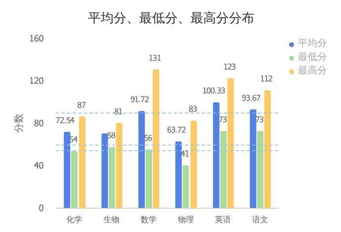
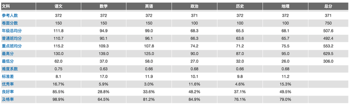
1、考情分析

　　各个科目的平均分、最高分、最低分是老师首先要考察的指标。以下图这个班级为例，对比各个科目的及格线分析，所有科目平均分都及格了，化学成绩比较突出，平均分达到了72.54，但是物理和生物成绩却不甚理想。三门主课里，英语的平均成绩较好，但是高分却一般。

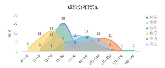
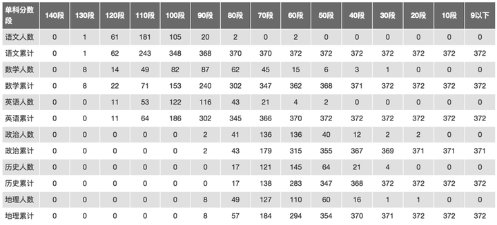
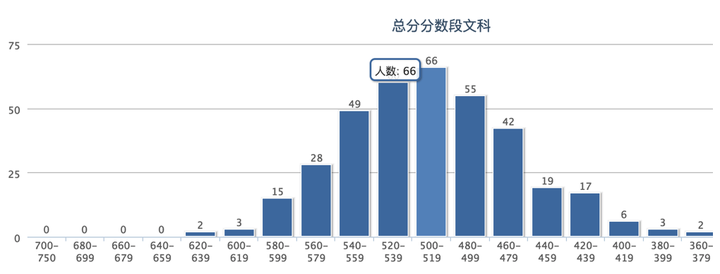
　　光凭上面的图还不能看出学生的整体水平，那么来看看频数分布图吧：

以10为单位对总分进行分段，统计各个分数段的频数，可以看出不同科目在各个分数段的人数分布，大致呈中间高两头低的拟正态分布曲线。

　　结果——真是远近高低各不同。物理成绩的波峰停留在61-70，说明大多数同学的成绩集中在这个分数段；化学在71-80分数段的人最多；数学的“山峰”最为绵延，分差较大；化学的“山峰”最陡峭，分差最小，大部分同学都及格了。

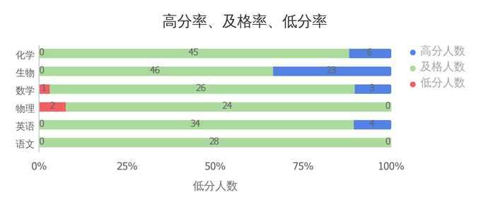
　　我们再以总分的40%、60%、80%分别设定低分线、及格线、高分线。总体来说，生物的高分人数最多，数学和物理落后的情况比较严重。综合以上结论，据我推测：

　　这可能是一个严重偏科的理科班，或者是一个分科后、会考前英语成绩比较好的文科班，也有可能只是考题太难，毕竟最高分都不理想。

　　（推理脸，严肃）

2、考试难度

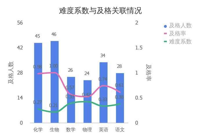
　　一切抛开试题看分数都是在耍流氓。考试考的不只是学生的掌握水平，还有老师的出题水平。那我们就来看看这次考试的难度系数：

　　难度系数是反映试题的难易程度的指标，难度系数越大自然考分就越低。难度系数这样来算：L=1—X/W其中，L为难度系数，X为样本平均得分，W为试卷总分。出（考）题（倒）无数的老师谈一点经验，试题的难度系数在0.3-0.7之间比较合适。

　　生物难度系数为0.21，试题偏简单，及格率达到100%。物理难度系数为0.42，属于中等难度，而及格率仅为52%，说明这个班级物理成绩的确有待加强。

　　其实，除了分析学生成绩之外，数据图表在平常的论文、报告、作业里也都适用的。

考试成绩分析案例：https://me.bdp.cn/share/index.html?shareId=sdo_a577450540c475cf4e7ccc9f1a6760d0 编辑于 2016-09-12 17:31赞同 16222 条评论分享收藏喜欢收起

知未105 人赞同了该回答

如何科学地分析学生成绩？就小学、初高中的学生成绩分析而言，应该有以下几个要素：

多层次：在年级、班级、学生、科目、题目多个层面上分别详细分析，并提供便利的下钻途径，逐层细化分析，探寻问题的根源，而不是停留在统计结果的表象。
多维度：从原始的题目维度，扩展到难度范围、知识点和考察能力，从多个维度上评估一个学生或班级的能力特征。
多次数：单独的一次考试受很多因素的影响，只有结合多次考试的数据进行动态分析，才能更加客观地评价。

接下来结合图表案例进行说明。

年级层面上，首先关心的是整个年级的整体情况，例如各科的参考人数，均分，最高最低，标准差，优秀良好及格的三率等等，这些数据让级长对本次考试的整体表现有个基本的了解。

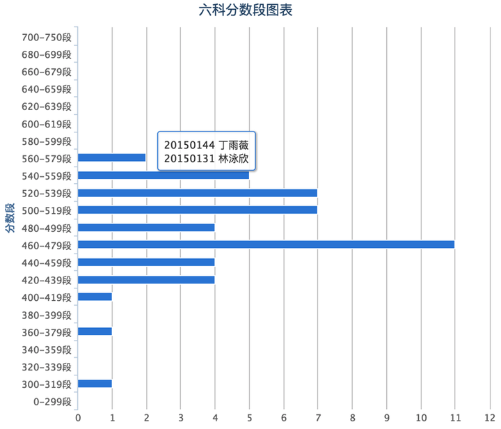
在年级总体均分的基础上，分析各分数段的人数，这样就对整个年级学生的分布有了直观认识，分布是否基本符合正态？是否有严重的两级分化？是否存在断层？

看完了整个年级的分数，接下来可以对各科目各班进行横向对比，通过均分柱图的比较，了解哪些班表现突出，哪些班落后于年级平均线。

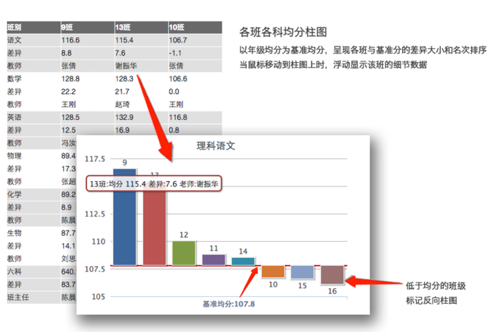
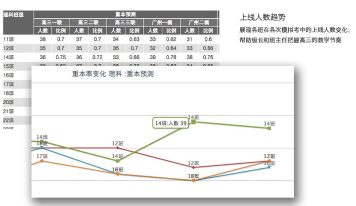
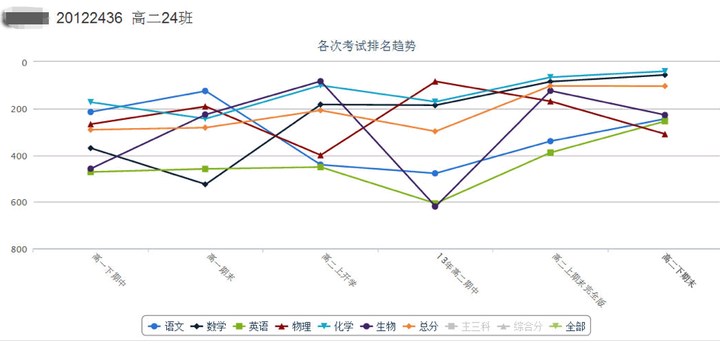
但更重要的是，是要进行纵向的分析，即和上一次考试的数据对比，了解各班的进退步情况，对于有进步的给予鼓励，退步的给予提醒，而不单纯只看本次的绝对值。

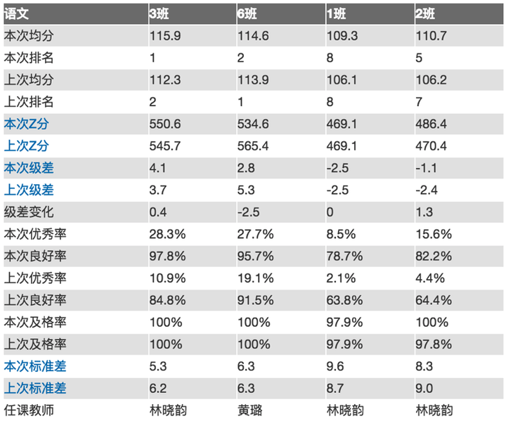
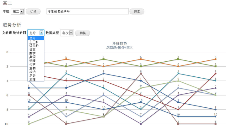
同样，我们也应该对每个班在历次考试中的各项数据表现都进行跟踪观察，才能科学评估班级的每次进退步的性质，给予合理的激励。

各班的均分体现的是一个班的整体表现，那这个班级内部的学生分布情况如何呢？可以利用学生名次构成分析来了解，也许两个班都是一样的均分，但其学生群体的分布大不相同，接下来采取的教学措施也就不一样了，有的重点可能是培优，有的重点可能是补差。

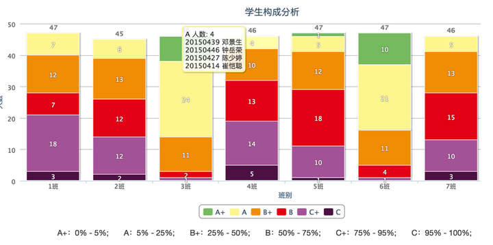
就培优而言，年级和各班班主任都首先会关注高分段学生的占比：

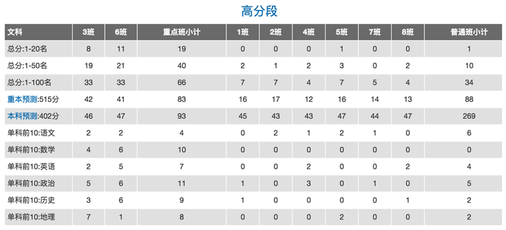
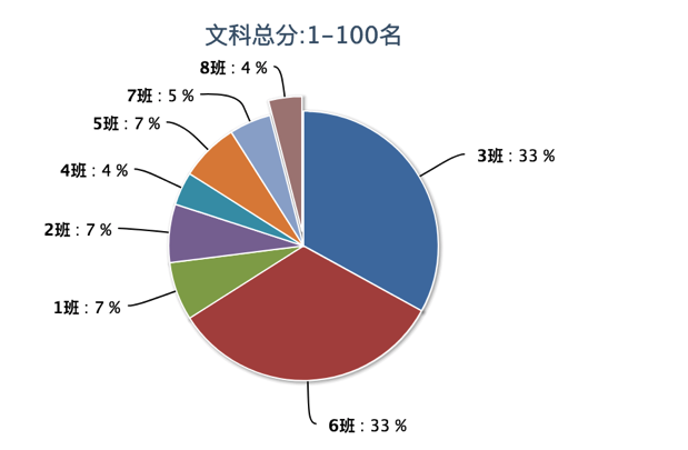
例子中的4班、8班，在前100名的人数过少，该班的培优工作有待改进。

而在高三年级，我们特别重视各个分数线的达标情况，对每次考试我们都应设立各重点线、本科线的标准，分析并跟踪各班上线人数的情况，对于落实年级的上线指标任务尤为重要。

年级层面可以关注的分析内容还有很多，但任何一个总体层面的分析，都是为了分解问题：整体的表现欠佳，是源自那些班级的因素最大？明确了这一点，我们就知道要重点抓哪个班的工作。

那这个班具体该怎么改进，这就引出了对单个班级的分析。

班主任和任课老师，可以在名次分布和分数分布两方面来了解本班学生的总体情况。

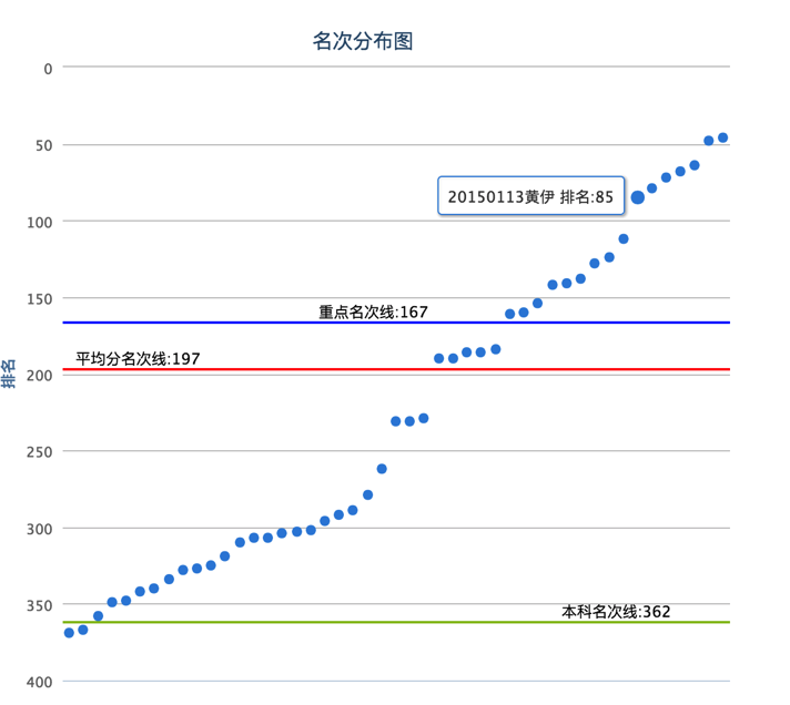
对于表现不佳的学生，或者需要重点关注的临界生，则应分析他历次考试的表现情况，和最近考试科目平衡性，找出最优先改进的科目：

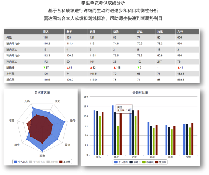
接下来就是针对该科目，详细分析他的题目层面的表现，了解该学生在哪些难度的题目上丢分较多，哪些知识点和考察能力较薄弱等等。

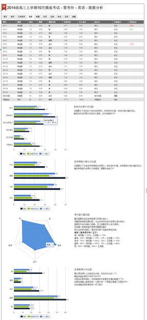
这些就是一个多层次、动态探究问题根源的完整过程，让一个年级层面的问题分解到一个学生具体的知识点层面的问题，把问题的解决落实到若干个可行的改进行动上，这样的分析最终才能产生教学质量进步的效果。也就是最前面提到的3要素：多层次、多维度、多次数；

要实现这样的分析体系，需要年级做到相应的准备工作：

1. 为每次考试收集详细的基础数据；

2. 建立合理的分析模型、采用高效率的分析工具；

3. 向全体师生分享数据，让大家在合理的权限控制下，适度参与分析，为自己的进步而分析。

这些工作有些是学校教务部门需要承担的，也有些可以采用外部的系统方案。目标只有一个，让每次考试所付出的时间和精力都得到回报，让考试产生的成绩数据，不仅用于正确地评价师生，更要给予师生们正确的反馈，引导师生进行有效的改进，从而实现教学质量的进步。

这些也是成绩云团队一直致力于实现的目标，我们希望扮演的就是这么一个高效的工具系统，协助学校实现改进教学质量的大目标。

成绩云chengjiyun.com/?from=zhihu